Have you met Julia Yet?

Table of Contents
Introduction
There are many different higher level programming languages out there such as C/C++, Go and Java which are probably considered more general computing languages or system languages.
There are more modern languages such as swift and kotlin which are very popular in app development.
Then there are higher level languages such as python, where the focus is simplicity and ease of use to allow the user to easily convert an idea or algorithm into program code.
There are also languages that have developed communities in specific fields such as R for data science.
For many years scientific computing was dominated by Fortran and MATLAB.
New languages are frequently added to the list and some slowly die off.
There are many more examples but what the long list of languages shows is that there is rarely a language that does everything well for the needs of a particular community.
For example, python is easy to learn and can do almost anything, but the trade off here is that it is an interpreted language and this makes it slow in comparison to Java and C which are compiled.
However, it’s ease of use has made it a star in recent years and the recent explosion in data science and AI has seen python’s popularity soar.
If you have come from a scientific or academic background, then you will probably have spent many years using MATLAB as it was (and still is) a staple of many science and engineering undergraduate courses.
And once you learn something you tend to keep using it because of familiarity: the devil you know is better than the one you don’t!
I fall into this last category, I learned of MATLAB as an undergraduate but couldn’t understand why we were being though something like this - who would ever need it?!
Roll on a few years into my Ph.D. and the first thing I did most days after switching on my computer was to open MATLAB in preparation for the days work.
I enjoyed using MATLAB as it made my life easier for reading big data files and doing all my calculations.
I couldn’t have managed without it really, but I always had a desire to find something that didn’t have a big price tag attached.
Something similar and familiar feeling but free so that I could use at home or in a future career.
I’d heard of this language called python that was like a cross between MATLAB and Perl and thought “This sounds good”, but I was nearing the end of my Ph.D. and the looming deadline meant I didn’t have time to explore.
Around the same time I also came across an announcement of a new language that sounded like my ideal language.
Like MATLAB to use but as fast as C. Perfect.
But it was new, and still under development. And my deadlines meant I soon forgot about it.
Eventually I moved on to python and have been well served by it for many years now.
But I still long for more speed at times. Particularly as my data sets grow with passing time (much like my waistline really).
Meet Julia
This is where I want to introduce Julia, which is still young.
Actually, looking at the date on the post, it’s 10 years exactly tomorrow! And that is a lot younger than python, which is approaching it’s 31st birthday very soon.
That early announcement sounded so intriguing to me, but I wasn’t prepared to spend a lot of time learning about a language that had yet to mature and show that it would be around long-term.
However, I must admit that I forgot about it for many years as python did such a good job of filling all the holes in my daily workflow.
Recently I picked up an old computer and logged in looking for some old files and saw the icon on the desktop for Julia.
It was time to look it up and see how it was doing. Had they fulfilled their initial greedy ambitions? Was it even still active?
As it turns out, Julia is alive and well, possibly even thriving as more and more people become aware of it.
I don’t want to write a tutorial on the use of Julia as there are already plenty of those, and many of which are quite detailed.
What I would like to do is just show a simple use case that highlights the power of Julia and why it’s worth your consideration.
Use Case: Vector Normalisation
Vector normalisation is possibly something that you would be doing frequently in scientific computing or some data processing. The most commonly encountered vector norm (often simply called “the norm” of a vector, or sometimes the magnitude of a vector)1 is the L2-norm, given by
$$ \left| x \right| _{2} = \left| x \right| = \sqrt{{x_{1}}^{2} + {x_{2}}^{2} + … + {x_{n}}^{2}} $$
This is a relatively simple calculation but can have a significant impact on performance if this is being calculated for a large number of vectors, partly because of the repeated use of a square root.
Test Environment
These are the details of the system on which I will do some test.
| System Specification | |
|---|---|
| Operating System | Windows 11 |
| Processor | Intel i9-9880H |
| Memory | 64GB |
| MATLAB Version | R2020a Update 5 |
| Python Version | Python 3.9.7 (default, Sep 16 2021, 16:59:28) [MSC v.1916 64 bit (AMD64)] |
| Julia Version | Version 1.7.2 (2022-02-06) |
MATLAB Implementation
I’ll start with the implementation in MATLAB, although there is already a norm and vecnorm function available in MATLAB.
However, It’s quite trivial to implement such a function in MATLAB (or any other language) using a simple for-loop to assign the result to some pre-allocated memory.
A second function using a vectorised approach is also implemented and can be compared with the inbuilt vecnorm function.
Performance is measured with the inbuilt timeit function2.
% define simple L2norm function
function norms = calc_norm_loop(vec_array)
    [m,n] = size(vec_array);
    norms = zeros(m);

    for i=1:m
        norms(i) = sqrt(sum(vec_array(i,:).^2));
    end

end

% vectorised
function norms = calc_norm(vec_array)
    norms = sqrt((sum(vec_array.^2, 2)));

end
A typical vector size of 50,000 3-component vectors is used for testing.
% create test set of vectors
vec_1 = rand(50000,3);

f = @() calc_norm_loop(vec_1); % handle to function
timeit(f)

f2 = @() calc_norm(vec_1); % handle to function
timeit(f2)

f3 = @() vecnorm(vec_1, 2, 2);
timeit(f3)

% check results
a = calc_norm_loop(vec_1);
b = calc_norm(vec_1);
c = vecnorm(vec_1, 2, 2);

% output in s
ans = 0.0153        % 15.3 ms
ans = 6.2837e-04    % 0.6283 ms
ans = 0.0021        % 2.1 ms
It’s not really a huge surprise to see that the for-loop implementation is the slowest by a large margin, but what is more interesting is that the vectorised function is actually many times quicker than the inbuilt function (I’ve repeated this test many times and the result is repeatable). I’m not quite sure why this is the case and it’s a little surprising to see an inbuilt function not fully optimised. It is possible it’s original purpose is for calculating the norm of vectors much longer than 3 elements and, as such, may not be optimised for my typical 3-component use case.
Python Implementation
Much like for MATLAB it’s quite trivial to implement such a function in native python with a for-loop but the numerical computing library NumPy provides a ready made solution for this3 in the Linear Algebra submodule and also provides the flexibility to calculate various other vector norms.
But if doing things in python quickly is something you want to do, you may also be interested in the Numba package.
The Numba package allows the user to significantly increase the performance of their code by pre-compiling the functions using a Just-In-Time (jit) compiler that runs the first time a function is called.
Once compiled, this function is then re-used, possibly offering significant performance gains for functions that are slow and called many times.
Here’s the implementation of both the native and Numba functions for calculating the L2-norm.
The interesting thing here is probably how little needs to be done to jit a function with Numba4 and unlock huge performance gains.
In this case, just one change is required - the addition of @njit() before the function. Super easy!!
import numpy as np
import math

from numba import njit

#%% Test functions - L2 Norm
# Native Python Implementation

def native_norm(vects):
    norms = []
    for vec in vects:
        norms.append(math.sqrt(vec[0]**2 + vec[1]**2 + vec[2]**2))

    return norms

# Numba Implementation
@njit()
def numba_norm(vects):
    norms = []
    for vec in vects:
        norms.append(math.sqrt(vec[0]**2 + vec[1]**2 + vec[2]**2))

    return norms
As many operations are size dependent, I’m going to use the perfplot package to helpfully run a benchmark suite of arrays of different sizes, from a single vector to a very large array of 3-component vectors.
out = perfplot.bench(
setup=lambda n: np.random.random([n,3]), # setup random nx3 array
kernels=[
lambda a: native_norm(a),
lambda a: np.linalg.norm(a, axis=1),
lambda a: numba_norm(a),
],
labels=["Native", "NumPy", "Numba"],
n_range=[2**k for k in range(25)],
xlabel="Number of vectors [Nr.]",
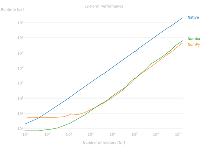
title="L2-norm Performance"
)
out.show(
time_unit="us", # set to one of ("auto", "s", "ms", "us", or "ns") to force plot units
)
This automates the whole process and creates a nice plot of the relative performance of the supplied function(s) which you can see in the figure below.
Numba function needs to be compiled before running the suite of benchmark tests or else the compilation time of the function is included. The function is compiled on first usage.
Some interesting takeaways from the results are:
- The native python implementation is the slowest (Not Surprising!)
- Numba is a powerful just-in-time compiler than can make your functions many times quicker. The jitted function is somewhere between 1 and 2 orders of magnitude quicker than the native
pythoncode. 50-100x faster for one line of code more! - As the array size increase, the
NumbaandNumPysolutions converge to the same results suggesting the code is being compiled to the same machine code.NumPyis slower for the smaller array sizes due to the overhead related to theNumPyfunction such as various implementation options and error checking. This overhead is large for the small array sizes but disappears for arrays above about several thousand rows in this. This is worth bearing in mind if you will only be working on small datasets.
Although, I’m using a specific package for my benchmarking, it’s really just automating the process of using timeit.
You will get very similar results running the following code for each size of array but this is a little tedious.
vects = np.random.random([100,3])

%timeit native_norms = native_norm(vects)
119 µs ± 1.61 µs per loop (mean ± std. dev. of 7 runs, 10000 loops each)

%timeit numpy_norms = np.linalg.norm(vects, axis=1)
6.72 µs ± 305 ns per loop (mean ± std. dev. of 7 runs, 100000 loops each)

%timeit numba_norms = numba_norm(vects)
1.96 µs ± 31.3 ns per loop (mean ± std. dev. of 7 runs, 1000000 loops each)
A more representative size for my typical use case would be much larger and, as shown in the figure, the gap between the NumPy and Numba implementations has disappeared at this size.
vects = np.random.random([50000,3])

%timeit native_norms = native_norm(vects)
59.5 ms ± 1.53 ms per loop (mean ± std. dev. of 7 runs, 10 loops each)

%timeit numpy_norms = np.linalg.norm(vects, axis=1)
920 µs ± 13.2 µs per loop (mean ± std. dev. of 7 runs, 1000 loops each)

%timeit numba_norms = numba_norm(vects)
841 µs ± 102 µs per loop (mean ± std. dev. of 7 runs, 1000 loops each)
Some interesting comparisons to the MATLAB results can be made with this set of figures for the larger test array size of 50,000 vectors. MATLAB’s for-loop is several times quicker than the native python loop, but both the NumPy and Numba implementations are quicker than vecnorm but slightly slower than the home-rolled vectorised function.
It’s worth pointing out that timeit returns the mean for python and the median for MATLAB.
I’ve also noticed that the MATLAB timing results are much less consistent as it only runs a small number of tests (just 11 in this case I think), so I’ve seen results range from 550 µs to 1.2 ms, putting it back in the same performance bracket as python when averaging these results.
Julia Implementation
Using Julia is a bit like writing code for python or MATLAB and it can be executed from the Julia REPL or using scripts.
Julia is in some sense acting a bit like Numba in that is is compiling all the code before execution to benefit from the performance gained from compiled code.
While I’m not yet aware of any perfplot equivalent for Julia just yet, it is relatively easy to measure the performance of any functions using the BenchmarkTools package.
I’m also going to use the LinearAlgebra and LoopVectorization packages to explore other options.
I’ve written the equivalent Julia function to my MATLAB and native python functions from earlier but in a vectorised manner as this is how I would write a similar function using Numpy.
Years of MATLAB/python exposure has “loops are bad” seared in my brain, but the results in the previous sections have demonstrated that is invariably the case in those languages.
using BenchmarkTools
using LinearAlgebra
using LoopVectorization

vec_1 = rand(50000,3)

function normalize_by_row(arr)
   sqrt.(sum(arr.^2, dims=2))
end
@btime provides a similar output to timeit, but it also includes the amount of memory used and number of memory allocations in the function.
Useful information for improving any function, however, it is returning the minimum execution time instead of the mean or median.
A more ‘full-fat’ option of @benchmark can also be used to get these metrics and other additional information.
julia> @btime nrm = normalize_by_row($vec_1);
  393.300 μs (10 allocations: 1.91 MiB)

julia> @benchmark nrm = normalize_by_row($vec_1)
BenchmarkTools.Trial: 7864 samples with 1 evaluation.
 Range (min … max):  378.100 μs …   7.246 ms  ┊ GC (min … max):  0.00% … 61.97%
 Time  (median):     454.300 μs               ┊ GC (median):     0.00%
 Time  (mean ± σ):   632.479 μs ± 628.993 μs  ┊ GC (mean ± σ):  19.93% ± 17.28%

  ▇█▆▅▄▃▂▂▁▁▁                                                   ▂
  ██████████████▇▇▇▆▆▄▄▄▃▁▄▃▁▃▁▃▁▁▁▃▁▁▁▁▁▄▄▄▅▅▅▅▇▇▇▇▇█▇▇▆▇▇▆▆▆▅ █
  378 μs        Histogram: log(frequency) by time       3.76 ms <

 Memory estimate: 1.91 MiB, allocs estimate: 10.
From this output we can see that our Julia function completes this operation on 50,000 3-component vectors over 7800 times with a median time of 454 μs and a mean time of 632 μs.
We can also see that our function is using about 2MB of memory to carry out this process.
So how did our MATLAB and python code perform for the same size array? Well if you remember, both were woefully slow in the for-loop but using the vectorised approach both were in the region of 800-900 μs.
Straight out of the box Julia outperforms both by a noticeable margin (20% or more) with little thought and zero optimisation required.
I’m already beginning to see a case for switching to using Julia…
But what about my initial Julia code? Can it be optimised like we did for MATLAB and python? What about all those memory allocations - do they make any difference to speed?
Let’s have a look at a few more possible options and see if there is a bit more performance to be gained.
Here’s the first attempt.
 function normalize_by_row_v2(arr)
    norms = Vector{Float64}(undef, size(arr)[1])
    temp = arr.^2
    for i in axes(arr,1)
       @views norms[i] = sqrt(sum(temp[i,:]))
    end

    return norms
 end

julia> @btime nrm = normalize_by_row_v2($vec_1);
  391.300 μs (4 allocations: 1.53 MiB)
This implementation looks quite different from the first attempt which was a simple broadcasted one-line solution.
This one has a loop!
It’s also using a temporary array for storage and the views function to reduce copying to memory.
Now here is the really interesting thing about Julia - even though I’ve reverted to a for-loop like tested earlier, performance has not been impacted at all.
In fact, this implementation has reduced memory usage and the number of memory allocations, making the code more memory efficient without slowing things down.
This is the really nice thing about using Julia: your code is automatically optimised!
Here’s another attempt at the one-liner with a subtle change from earlier that does improve the performance and it’s quite a significant jump.
Julia is now approximately 3-5 times quicker than MATLAB and python.
function normalize_by_row_v3(arr)
    sqrt.(sum(x->x^2,arr, dims=2))
end

julia> @btime nrm = normalize_by_row_v3($vec_1);
  138.300 μs (8 allocations: 781.42 KiB)
So now you must be thinking “we have not done much yet, maybe we can optimise this function more?". To try and ‘scratch that itch’ I’ve gone thorough the docs, watched a few youtube videos and scoured some of the popular user forums and come up with a few possible options. If it is possible to squeeze more performance, how much better can we do?
Are loops really that bad?
So I briefly mentioned this idea that loops are bad and you may be familiar with this concept if you are coming from python and MATLAB, where the for-loop option is often many times slower than the vectorised approach.
But in my few examples, I’ve just demonstrated that this isn’t the case in Julia where a loop can achieve the same performance as the vectorised approach.
This is because all code is statically typed and then compiled, much like Fortran, C or Java and not interpreted like MATLAB or python.
This static typing and compilation allows much more performance to be extracted as all the information is known beforehand and the compiler can then optimise the code into fast machine code whereas in interpreted languages there is a constant need to check everything as type information is often missing and then it needs to be translated into machine code at runtime.
Packages like NumPy provide highly optimised functions that are actually compiled to C beforehand, hence their performance.
I think that’s partly where this “loops are bad” mentality comes from: in an interpreted language there are quick vectorised libraries that you can use and they are quicker than something that will be compiled into bytecode by the python compiler for example.
So let’s see how we can optimise our Julia code by passing some additional instructions to the compiler to help it.
 function normalize_by_row_v4(arr)
    norms = Vector{Float64}(undef, size(arr)[1])
    @inbounds for i in axes(arr, 1)
        anorm2 = zero(eltype(arr))
        for j in axes(arr, 2)
            anorm2 += arr[i, j]^2
        end
        norms[i] = sqrt(anorm2)

    end
    return norms
end

julia>  @btime nrm = normalize_by_row_v4($vec_1);
  91.700 μs (2 allocations: 390.67 KiB)
Wow! So we have found another 30% reduction in from our best performing method so far but actually about 4x quicker than our previous looped example.
It’s also possible to use the LoopVectorization package to enable some extra optimisations during the compilation process.
Always verify that these optimisations don’t affect the results from your calculations as they may be doing something like changing the order of calculations.
You have been warned!
using LoopVectorization

function normalize_by_row_v4_turbo(arr)
    norms = Vector{Float64}(undef, size(arr)[1])
    @turbo for i in axes(arr, 1)
        anorm2 = zero(eltype(arr))
        for j in axes(arr, 2)
            anorm2 += arr[i, j]^2
        end
        norms[i] = sqrt(anorm2)

    end
    return norms
end

julia>  @btime nrm7 = normalize_by_row_v4_turbo($vec_1);
  40.300 μs (2 allocations: 390.67 KiB)
Another wow! By using the LoopVectorization package we can give the @turbo instruction to the compiler which really does add some turbo!!
So there you have it, proof that loops are not bad! Our optimised Julia function has blown python and MATLAB out of the water and is now about 10-15x faster.
This was a relatively simple use case but highlights even for something simple there are possibly significant gains to be made.
As I mentioned earlier Julia is still young but it appears to be reaching a point where it’s difficult to ignore it any more.
There is no doubting it’s fast, it’s on the same level as C, C++ and Fortran and is a member of the Petaflop Club having achieved 1.54 petaflops with 1.3 million threads on the Cray XC40 supercomputer5.
Summary
One line summary - If you want to make your python code 10x times quicker use Julia!!
Well that’s not really been the point of this post, but it is eye catching. 10x speedup is a lot.
But there’s more to Julia than just speed. It has an interactive REPL just like python, it is supported by Jupyter notebooks and has it’s own interactive notebooks called Pluto which I think are actually far superior. Want multi-threading? Done!
Julia was created by MATLAB and python users so there will be a somewhat familiar feel to those making the transition.
There is also a growing eco-system that allows users start on tasks like solving lots of differential equations or machine learning without much development required by the user.
I’m very impressed by where Julia has ended up after 10 years and it’s something I seriously consider now every time I am starting a new project as there is still some inertia in shifting completely from one language to a new one.
I don’t know if I will ever completely switch, but I do know I’m going to be using Julia a lot more in the future to reduce some of my computing bottlenecks in some tasks.
Have you seen enough to tempt you into getting to know Julia a bit better?
References
-
Weisstein, Eric W. “Vector Norm.” From MathWorld–A Wolfram Web Resource. https://mathworld.wolfram.com/VectorNorm.html. Accessed on 13/2/2022 ↩︎
-
Eddins, Steve. “timeit makes it into MATLAB”. https://blogs.mathworks.com/steve/2013/09/30/timeit-makes-it-into-matlab/?doing_wp_cron=1645382790.6918818950653076171875. Accessed on 13/2/2022 ↩︎
-
NumPy API Reference. https://numpy.org/doc/stable/reference/generated/numpy.linalg.norm.html#rac1c834adb66-1. Accessed on 13/2/2022 ↩︎
-
Numba Quickstart Guide. https://numba.pydata.org/numba-doc/latest/user/5minguide.html. Accessed on 13/2/2022 ↩︎
-
“Julia Joins Petaflop Club”. https://www.hpcwire.com/off-the-wire/julia-joins-petaflop-club/. Accessed on 13/2/2022 ↩︎
John P. Morrissey
Research Scientist in Granular Mechanics
My research interests include particulate mechanics, the Discrete Element Method (DEM) and other numerical simulation tools. I’m also interested in all things data and how to extract meaningful information from it.